Double-Slit: Healing Hemispheres → Detector Distance Test
Two healed hemispherical emitters at the slits radiate forward. We compute detector intensity at distance L by coherent summation and automatically compare measured peak rows to analytic maxima. Controls scan geometry and wave parameters so you can verify that detected fringes move exactly as CBF predicts from phase alignment at the screen.
How this maps to CBF
Slit edges spawn **healing hemispheres**. This demo instantiates two hemispherical emitters at the slits and streams many pulses (photons) forward. As fronts advance, their phase evolves. The detector does not accumulate “overlap energy,” it tests for **phase alignment at the screen**, which stands in for the Event Ledger’s temporal gate. Commit frequency appears as bright rows, while misaligned rows remain dark. The analytic comparison visualizes the Ledger’s additional geometric consistency checks.
What to expect on the detector
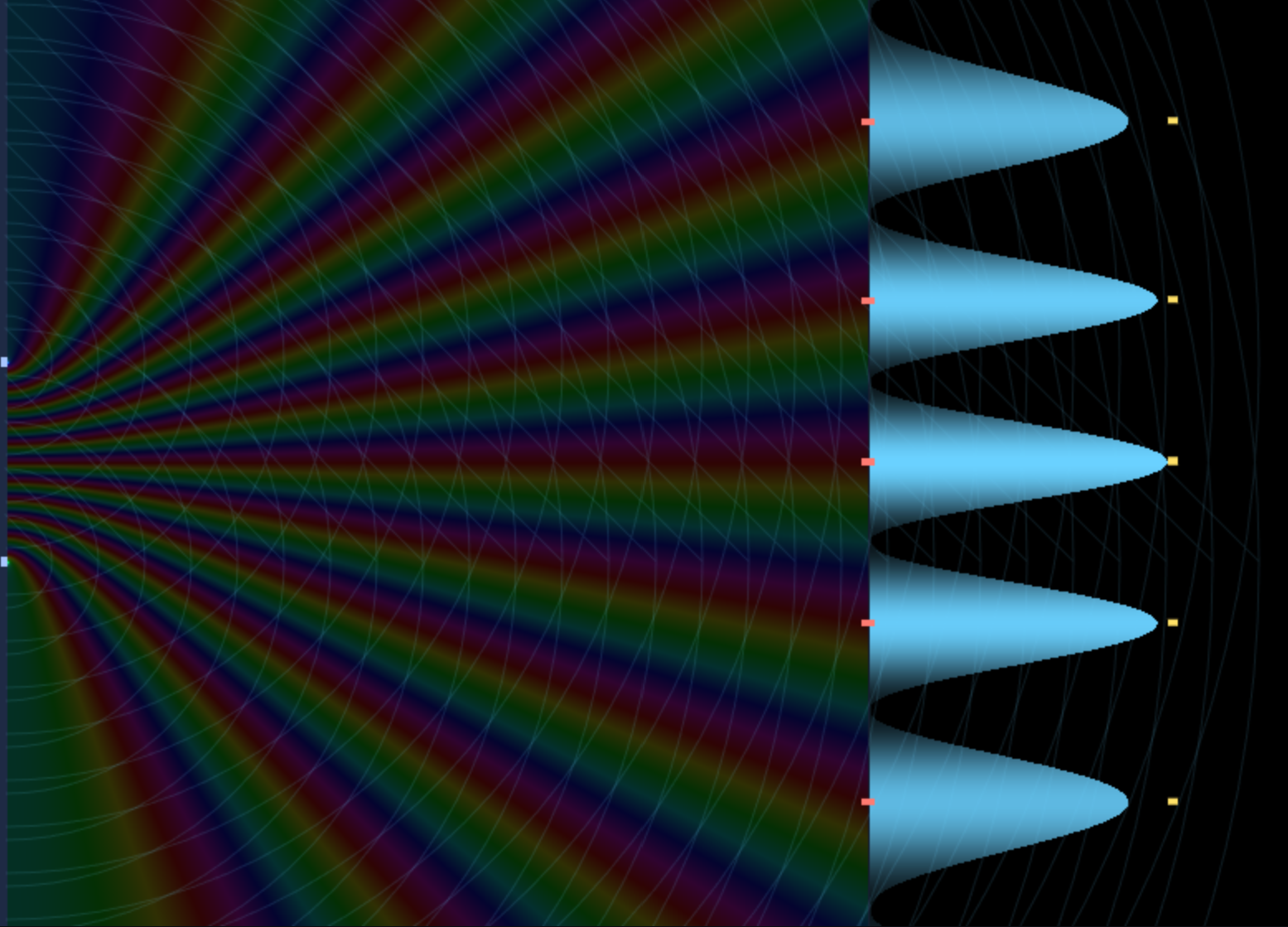
As the wavefronts reach the detector, the centerline arrives with relatively steady phase, while the off-axis regions experience faster phase rotation due to path-length differences. The screen is not the same color all the way down: near the edges, the phase flips multiple times before the bulk arrives, creating alternating bright and dark bands. Scanning L, d, and λ moves these bands exactly as predicted by m λ = d sinθ.
The colored finger-like bands show the running history of where commits were likely to occur, a probability trace of potential events along the screen.
Settings
| Parameter | Default | Notes |
|---|---|---|
| Detector distance L | 520 px | Moves screen to test far/near field. |
| Slit separation d | 120 px | Sets fringe spacing scale, mλ = d sinθ. |
| Wavelength λ | 22 px | Changes k = 2π/λ, shifting all phases. |
| Detector height H | 560 px | Canvas height and sample rows. |
| Front spacing (draw) | 28 px | Visual phase-front density only. |
| Fronts show wavelength | off | Use half-λ front spacing when on. |
| Peak threshold | 0.25 | Fixed or adaptive if too few peaks. |
| Max order m to score | 10 | Restricts analytic maxima considered. |
| Pass tolerance (px) | 3 px | Absolute error pass line. |
| Pass tolerance (fraction) | 0.25 | Local-spacing normalized pass line. |
| Color fringes | off | Optional phase-colored propagation field. |
Key Code
This routine builds the screen intensity by summing complex contributions from two **hemispherical** sources located at
y = ±d/2, evaluated along the detector at x = L. Each source uses a simple transport factor
1/r and phase k r, then we square the magnitude of the phasor sum to get the intensity row.
We support optional sub-pixel supersampling when predicted fringe spacing becomes too small for the current detector sampling, to avoid aliasing under extreme geometry. This keeps the peak locations faithful for later matching against the analytic formula.
Healing hemispheres: CBF says slit edges seed hemispherical healing. Here, each slit is represented as a hemispherical emitter. We do not run the full healing solver, but the geometry and phase law capture the essential **direction diversification** and **path-length** differences that feed the Ledger.
Temporal gate proxy: The phasor sum at the detector stands in for the Event Ledger’s temporal gate, which accepts commits where phases beat-match. The returned |E|² per row is the commit-frequency statistic, not a pre-screen energy overlap.
We predict maxima rows using the standard double-slit condition m λ = d sinθ, convert angles to row offsets, and keep
only orders that appear on the current detector. Measured peaks are found via a robust detector with a fixed threshold or a backup
adaptive threshold. We then match analytic rows to measured peaks on the same side of the centerline with a local search window.
To report accuracy, we compute mean absolute error in pixels and a **fractional error** normalized by the local fringe spacing around each order, which stabilizes the score across varying geometries. Pass/fail uses the tighter of absolute and fractional tolerances.
Constraint-checked commits: Matching measured peaks to analytic orders is the visualization of the Ledger’s **spatial gate** meeting the **temporal gate**. If phases do not reconcile to the allowed geometry, no commit is counted there.
Local fairness: Normalizing by **local fringe spacing** mirrors CBF’s idea that acceptance should be judged in the context of nearby viable outcomes, not in absolute pixel units that vary with L, d, and λ.
The draw pass renders the slit wall and the two seed points, then either evenly spaced fronts (for clarity) or wavelength-spaced phase fronts. When “Color fringes” is enabled, we compute the local interference field between the wall and detector and color by phase while modulating lightness by instantaneous intensity.
Detector output is drawn as horizontal bars proportional to intensity, with **yellow** markers for measured peaks, and **red** ticks for analytic maxima. This side-by-side view makes it obvious when parameters force peaks in or out of frame and helps debug thresholding, sampling, or extreme geometries.
Phase as visible ledger input: Phase-fronts and the colored field make the incoming information to the Ledger explicit, so you can see why the screen accepts more commits at certain rows.
Outcome vs. mechanism: You never “see waves” in CBF, you see accepted commits. The detector bars and peak markers are the outcomes; the colored field is there so we can understand why those outcomes appear.