Redshift: Pacing Ratio, No Photon Buffer
This demo shows how observed frequency and temperature scale with the **pacing ratio**. For photons in CBF, M = 0 (no temporal queue), so the wavelength history is read at detection via the local pacing factor α.
Core relations: f_obs = f_emit × (α_obs / α_emit) and
1 + z = α_emit / α_obs, so T_now = T_emit / (1+z).
How this maps to CBF
In CBF, photons carry no maintenance budget (M = 0) and therefore do not build a temporal queue. Their frequency never changes in flight. What we call redshift arises only when the detector reads the frozen oscillation pattern through a different local pacing factor, \( \alpha \).
The pacing factor \( \alpha(x) \) sets how fast local clocks run relative to the universal baseline. It reflects how much of each tick’s causal budget is devoted to translation versus maintenance: \( \alpha = T / (T + M) \). Regions with deeper gravitational potential, higher curvature, or slower local clock rate have smaller \( \alpha \); low-gravity or later-epoch regions have larger \( \alpha \).
This single mechanism unifies gravitational and cosmological redshift: both are simply differences in \( \alpha \) between emission and observation points. For a photon emitted at \( \alpha_{\text{emit}} \) and detected at \( \alpha_{\text{obs}} \), \( f_{\text{obs}} = f_{\text{emit}} \times (\alpha_{\text{obs}} / \alpha_{\text{emit}}) \), and equivalently \( 1 + z = \alpha_{\text{emit}} / \alpha_{\text{obs}} \).
Photons propagate with \( C = T \) only. The observed frequency depends entirely on how the observer’s local pacing \( \alpha_{\text{obs}} \) reads the emission pattern written at \( \alpha_{\text{emit}} \). Thus gravitational redshift near a massive body and cosmological redshift across expanding epochs are two expressions of the same pacing-ratio rule.
Photons as Pacing Snapshots
In CBF, a photon is not an energy packet. It is a pacing snapshot of an oscillation pattern. Think of a vinyl record: the grooves are fixed at pressing, and the music you hear depends on the record player’s RPM. Likewise, a photon’s pattern is fixed at emission, and what you “hear” at detection depends on the local pacing.
- At emission: The atom’s current \( C = T + M \) at \( \alpha_{\text{emit}} \) is imprinted into the oscillation pattern. In CBF, oscillation arises from atom \(T+M\) vibration, so IR/visible/UV is literally the pattern produced by that budget at that moment.
- In transit: No internal clock, no buffering, no evolution. Photons have \( M = 0 \), so the same pattern simply propagates.
- At detection: The observer’s current \( C = T + M \) at \( \alpha_{\text{obs}} \) reads that pattern. The playback rate rescales by the pacing ratio \( f_{\text{obs}} = f_{\text{emit}} \times (\alpha_{\text{obs}} / \alpha_{\text{emit}}) \). Thus, “IR at emitter” need not remain IR at detector.
A thermal field’s Planck distribution encodes the emitter’s state. When read at a different pacing, the entire spectrum shifts coherently: \( T_{\text{now}} = T_{\text{emit}} \times (\alpha_{\text{obs}} / \alpha_{\text{emit}}) = T_{\text{emit}}/(1+z) \).
CBF does not conserve “photon number.” Each emission is a local ledger transaction converting stored \( M \) into propagating \( T \). What is conserved is the total causal budget \( C \), not a particle inventory.
Interference is superposition at the reconciliation layer: overlapping field commits whose phases are compared when events are added to the ledger. No self-interfering particles are required.
What to expect
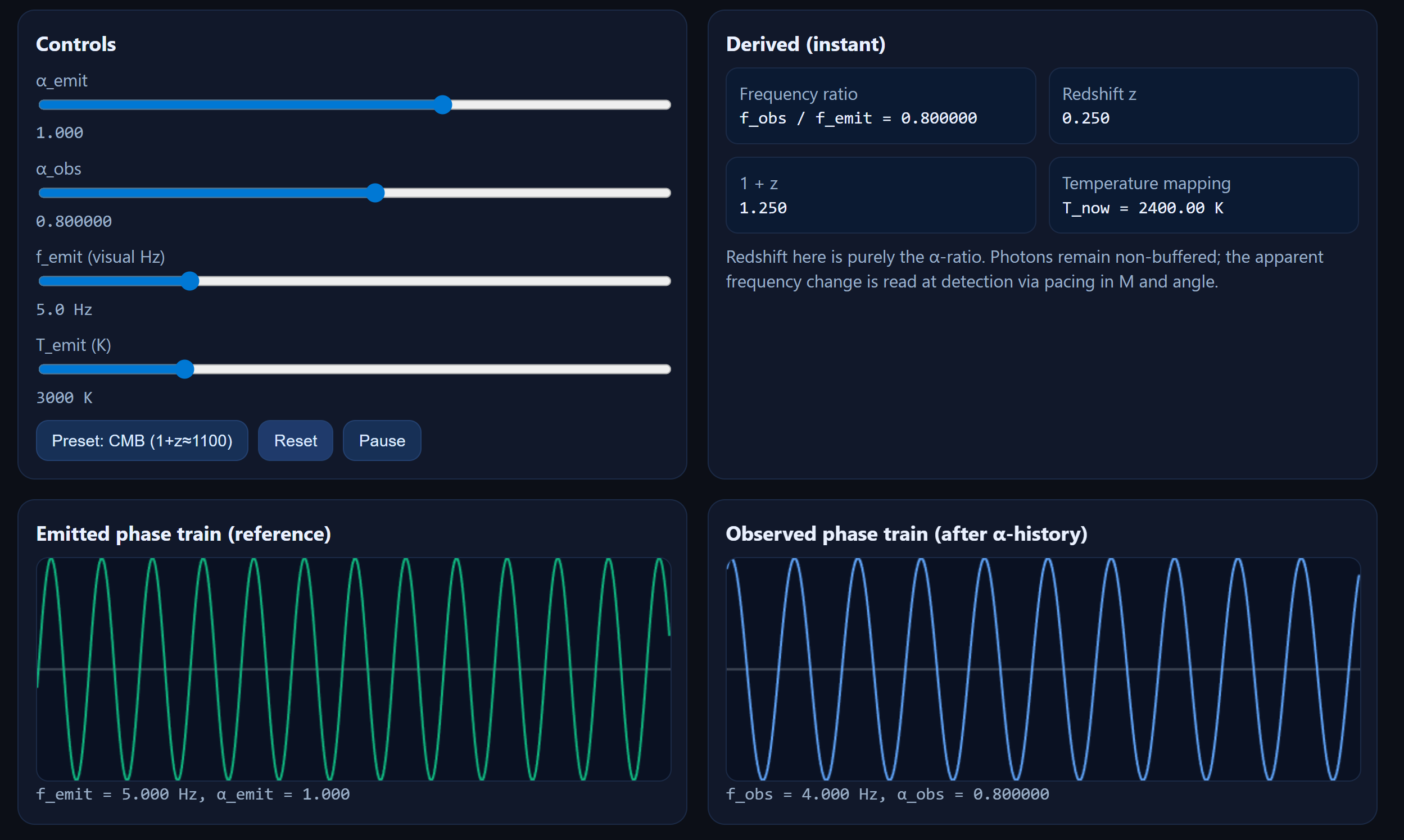
- Live ratios: As you slide α_emit and α_obs, the panel updates
f_obs / f_emit,z,1+z, andT_nowinstantly. - Phase trains: The emitted canvas shows the reference oscillation at
f_emit. The observed canvas shows the resampled train atf_obs. - CMB preset: Tap “Preset: CMB (1+z≈1100)” to visualize the scaling from recombination to now,
using
α_emit = 1andα_obs = 1/1100. - Interference tab: A second tab illustrates that interference comes from the field’s phase comparison, not from stored photon phase history.
Key Code
This function computes the pacing-based scaling used throughout the UI. It implements
f_obs = f_emit × (α_obs / α_emit),
1+z = f_emit / f_obs, and
T_now = T_emit / (1+z).
Pacing ratio at commit: The detector samples the passing wave with its local clock. Changing α changes the sample rate, which appears as a different observed frequency and, for a thermal source, a rescaled temperature label.
Two canvases render side-by-side oscillations. The observed one is not “stretched in flight,”
it is simply drawn at the detector’s sampled rate f_obs.
No temporal storage: The observed plot is a live readout at the detector’s pace. This visualizes the “no photon buffering” rule: the phase history is reconciled at the boundary, not carried as an internal queue.
The CMB preset uses α_emit = 1 and α_obs = 1/1100 for a quick visual of recombination-to-now scaling.
Sliders update state and refresh the derived panel and plots.
Cosmic scaling: The CMB preset is an illustration of reading a very old phase label at a much slower local clock. In CBF terms, the long flight does not accumulate a buffer, the redshift appears when the Event Ledger compares pacing at commit.